Welcome to CVsim!

# Uncomment and run below command if you're running the notebook locally and need to install cvsim.

#!pip install cvsim

import numpy as np
import matplotlib.pyplot as plt
from cvsim.mechanisms import E_rev, E_q, E_qC, EE, SquareScheme
from cvsim.fit_curve import FitE_rev, FitE_q, FitE_qC, FitEE, FitSquareScheme

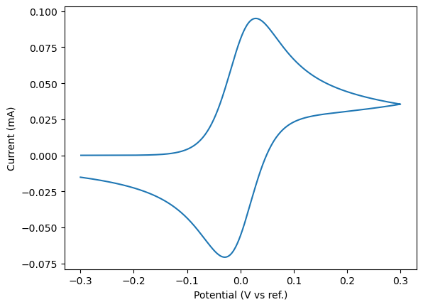
Example: Reversible, one-electron mechanism

potential, current = E_rev(
    start_potential=-0.3,     # V vs ref.
    switch_potential=0.3,     # V vs ref.
    reduction_potential=0.0,  # V vs ref.
    scan_rate=0.1,            # V/s
    c_bulk=5,                 # mM
    diffusion_reactant=1e-5,  # cm2/s
    diffusion_product=1e-5,   # cm2/s
).simulate()

fig, ax = plt.subplots()
ax.plot(potential, current*1000)
ax.set_xlabel('Potential (V vs ref.)')
ax.set_ylabel('Current (mA)')

Text(0, 0.5, 'Current (mA)')

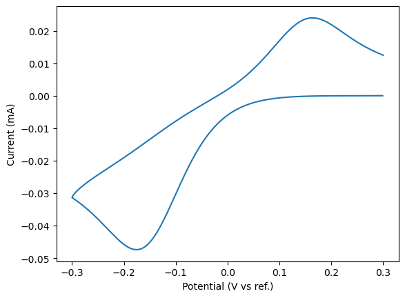
Example: Quasi-reversible, one-electron mechanism

potential, current = E_q(
    start_potential=0.3,      # V vs ref.
    switch_potential=-0.3,    # V vs ref.
    reduction_potential=0.0,  # V vs ref.
    scan_rate=1,              # V/s
    c_bulk=1,                 # mM
    diffusion_reactant=1e-5,  # cm2/s
    diffusion_product=1e-5,   # cm2/s
    alpha=0.5,                # unitless
    k0=1e-3,                  # cm/s
).simulate()

fig,ax = plt.subplots()
ax.plot(potential, current*1000)
ax.set_xlabel('Potential (V vs ref.)')
ax.set_ylabel('Current (mA)')

Text(0, 0.5, 'Current (mA)')

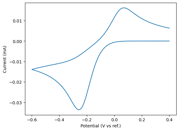
Example: The EC mechanism

potential, current = E_qC(
    start_potential=0.4,       # V vs ref.
    switch_potential=-0.6,     # V vs ref.
    reduction_potential=-0.1,  # V vs ref.
    scan_rate=0.5,             # V/s
    c_bulk=1,                  # mM
    diffusion_reactant=1e-5,   # cm2/s
    diffusion_product=1e-5,    # cm2/s
    alpha=0.5,                 # unitless
    k0=1e-3,                   # cm/s
    k_forward=0.01,            # 1/s
    k_backward=0.015,          # 1/s
).simulate()

fig,ax = plt.subplots()
ax.plot(potential, current*1000)
ax.set_xlabel('Potential (V vs ref.)')
ax.set_ylabel('Current (mA)')

Text(0, 0.5, 'Current (mA)')

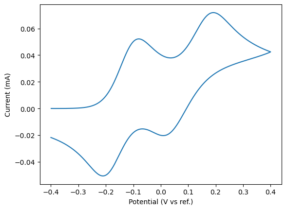
Example: The EE mechanism

potential, current = EE(
    start_potential=-0.4,         # V vs ref.
    switch_potential=0.4,         # V vs ref.
    reduction_potential=-0.15,    # V vs ref.
    reduction_potential2=0.1,     # V vs ref.
    scan_rate=1.0,                # V/s
    c_bulk=1,                     # mM
    diffusion_reactant=1e-5,      # cm2/s
    diffusion_intermediate=1e-5,  # cm2/s
    diffusion_product=1e-5,       # cm2/s
    alpha=0.5,                    # unitless
    alpha2=0.5,                   # unitless
    k0=1e-2,                      # cm/s
    k0_2=5e-3,                    # cm/s
).simulate()

fig,ax = plt.subplots()
ax.plot(potential, current*1000)
ax.set_xlabel('Potential (V vs ref.)')
ax.set_ylabel('Current (mA)')

Text(0, 0.5, 'Current (mA)')

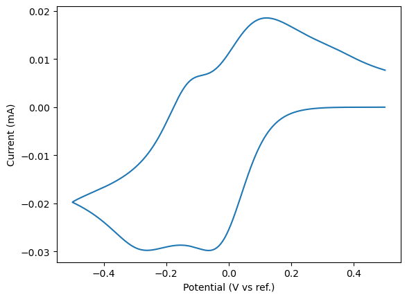
Example: The Square Scheme mechanism

potential, current = SquareScheme(
    start_potential=0.5,        # V vs ref.
    switch_potential=-0.5,      # V vs ref.
    reduction_potential=0.2,    # V vs ref.
    reduction_potential2=-0.2,  # V vs ref.
    scan_rate=1.0,              # V/s
    c_bulk=1,                   # mM
    diffusion_reactant=1e-5,    # cm2/s
    diffusion_product=1e-5,     # cm2/s
    alpha=0.5,                  # unitless
    alpha2=0.5,                 # unitless
    k0=1e-3,                    # cm/s
    k0_2=5e-3,                  # cm/s
    k_forward=0.3,              # 1/s
    k_backward=0.1,             # 1/s
    k_forward2=0.01,            # 1/s
    k_backward2=0.002,          # 1/s
).simulate()

fig,ax = plt.subplots()
ax.plot(potential, current*1000)
ax.set_xlabel('Potential (V vs ref.)')
ax.set_ylabel('Current (mA)')

Text(0, 0.5, 'Current (mA)')

Fitting CVs

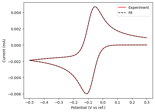
Example: fit the E_rev mechanism

# if you don't have real CV data to fit, make "fake" data here via CVsim
fake_voltages, fake_currents = E_rev(0.3, -0.5, -0.1, 0.1, 1, 1e-6, 4e-6).simulate()
# add data point at zero current
fake_voltages = np.insert(fake_voltages, 0, 0.3)
fake_currents = np.insert(fake_currents, 0, 0.0)

# fit the "experimental" data
fitted_voltage, fitted_current, final_fit = FitE_rev(
    voltage_to_fit=fake_voltages,  # list, V vs ref.
    current_to_fit=fake_currents,  # list, A
    scan_rate=0.1,                 # V/s
    c_bulk=1,                      # mM
    step_size=1,                   # mV
    disk_radius=1.5,               # mm
    temperature=298,               # K
).fit()

fig, ax = plt.subplots()
ax.plot(fake_voltages, fake_currents*1000, 'r', label="Experiment")
ax.plot(fitted_voltage, fitted_current*1000, 'k--', label="Fit")
ax.legend()
ax.set_xlabel('Potential (V vs ref.)')
ax.set_ylabel('Current (mA)')

final fitting vars: {'reduction_potential': [-0.082, -0.5, 0.3], 'diffusion_reactant': [1e-06, 5e-08, 0.0001], 'diffusion_product': [1e-06, 5e-08, 0.0001]}
Initial guesses: (-0.082, 1e-06, 1e-06)
Lower/Upper bounds: (-0.5, 5e-08, 5e-08)/(0.3, 0.0001, 0.0001)
Fixed params: []
Fitting for: ['reduction_potential', 'diffusion_reactant', 'diffusion_product']
trying values: (-0.082, 1e-06, 1e-06)
trying values: (-0.0820000149011612, 1e-06, 1e-06)
trying values: (-0.082, 1.0149011611938476e-06, 1e-06)
trying values: (-0.082, 1e-06, 1.0149011611938476e-06)
trying values: (-0.082, 1e-06, 1e-06)
Final fit: 'reduction_potential': -8.20E-02 +/- 2E-03
Final fit: 'diffusion_reactant': 1.00E-06 +/- 1E-10
Final fit: 'diffusion_product': 1.00E-06 +/- 2E-07

Text(0, 0.5, 'Current (mA)')

# access final fit parameters
final_fit

{'reduction_potential': -0.082,
 'diffusion_reactant': 1e-06,
 'diffusion_product': 1e-06}

A word of caution: different diffusion coefficient values still give the same CV under E_rev conditions (the beauty of Nernstian kinetics!).

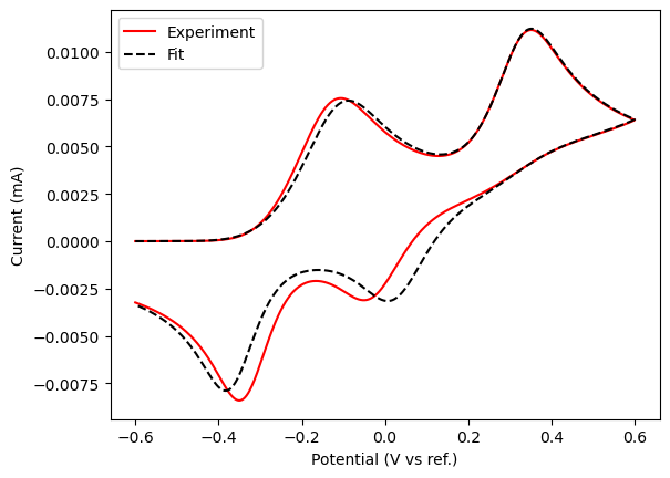
Example: fit the EE mechanism, now with some known priors

We will assume that diffusion/transfer coefficients were obtained experimentally from an RDE experiment, and an educated guess for the ranges of electrochemical rate constants is known.

# again we'll make "fake" data here via CVsim
fake_voltages, fake_currents = EE(-0.6, 0.6, -0.25, 0.15, 0.1, 1, 3e-6, 3e-6, 3e-6, 0.4, 0.5, 5e-4, 1e-4).simulate()
# add data point at zero current
fake_voltages = np.insert(fake_voltages, 0, -0.6)
fake_currents = np.insert(fake_currents, 0, 0.0)

# fit the "experimental" data
fitted_voltage, fitted_current, final_fit = FitEE(
    voltage_to_fit=fake_voltages,  # list, V vs ref.
    current_to_fit=fake_currents,  # list, A
    diffusion_reactant=3e-6,       # cm2/s, known prior
    diffusion_intermediate=3e-6,   # cm2/s, known prior
    diffusion_product=3e-6,        # cm2/s, known prior
    alpha=0.4,                     # unitless, known prior
    alpha2=0.5,                    # unitless, known prior
    scan_rate=0.1,                 # V/s
    c_bulk=1,                      # mM
    step_size=1,                   # mV
    disk_radius=1.5,               # mm
    temperature=298,               # K
).fit(
    # here is where we input guesses and/or ranges for guesses
    reduction_potential=-0.3,
    reduction_potential2=0.2,
    k0=(2e-4, 1e-4, 2e-3),
    k0_2=(3e-4, 5e-5, 5e-4),
)

final fitting vars: {'reduction_potential': [-0.3, -0.6, 0.6], 'reduction_potential2': [0.2, -0.6, 0.6], 'k0': [0.0002, 0.0001, 0.002], 'k0_2': [0.0003, 5e-05, 0.0005]}
Initial guesses: (-0.3, 0.2, 0.0002, 0.0003)
Lower/Upper bounds: (-0.6, -0.6, 0.0001, 5e-05)/(0.6, 0.6, 0.002, 0.0005)
Fixed params: ['diffusion_reactant', 'diffusion_product', 'diffusion_intermediate', 'alpha', 'alpha2']
Fitting for: ['reduction_potential', 'reduction_potential2', 'k0', 'k0_2']
trying values: (-0.3, 0.2, 0.0002, 0.0003)
trying values: (-0.3000000149011612, 0.2, 0.0002, 0.0003)
trying values: (-0.3, 0.2000000149011612, 0.0002, 0.0003)
trying values: (-0.3, 0.2, 0.00020001490116119386, 0.0003)
trying values: (-0.3, 0.2, 0.0002, 0.0003000149011611938)
trying values: (-0.26305206966930683, 0.17758408428413522, 0.00030812615917673596, 0.00016803814477157466)
trying values: (-0.263052084570468, 0.17758408428413522, 0.00030812615917673596, 0.00016803814477157466)
trying values: (-0.26305206966930683, 0.1775840991852964, 0.00030812615917673596, 0.00016803814477157466)
trying values: (-0.26305206966930683, 0.17758408428413522, 0.0003081410603379298, 0.00016803814477157466)
trying values: (-0.26305206966930683, 0.17758408428413522, 0.00030812615917673596, 0.0001680530459327685)
trying values: (-0.26305206966930683, 0.17758408428413522, 0.00030812615917673596, 0.00016803814477157466)
Final fit: 'reduction_potential': -2.63E-01 +/- 8E-04
Final fit: 'reduction_potential2': 1.78E-01 +/- 9E-04
Final fit: 'k0': 3.08E-04 +/- 5E-06
Final fit: 'k0_2': 1.68E-04 +/- 3E-06

fig, ax = plt.subplots()
ax.plot(fake_voltages, fake_currents*1000, 'r', label="Experiment")
ax.plot(fitted_voltage, fitted_current*1000, 'k--', label="Fit")
ax.legend()
ax.set_xlabel('Potential (V vs ref.)')
ax.set_ylabel('Current (mA)')

Text(0, 0.5, 'Current (mA)')

# access final fit parameters
final_fit

{'reduction_potential': -0.26305206966930683,
 'reduction_potential2': 0.17758408428413522,
 'k0': 0.00030812615917673596,
 'k0_2': 0.00016803814477157466}

The fit method can optionally receive: a float for an initial guess of the parameter; tuple[float, float] for (lower bound, upper bound) of the parameter; or tuple[float, float, float] for (initial guess, lower bound, upper bound).